Lecture 13/14
Probability Distributions for Continous Random Variables
Section 6.1 Probability Distributions for Continuous Random Variables
Last time we talked about discrete random variables - there was a probability associated with each value.
For example, there was a set count of possible laptops sold at the store:
\[ P(x = 3) = .15 \]
We could also answer the questions of what is the probability of at least 3 laptops being sold.
For example:
\[ P(x \ge 3) = .15 + .1 + .05 = .3 \]
What if, instead, I observed a variable that was continuous.
For example: temperature, height, rainfall
A continuous variable can sometimes look discrete because of imprecision in measurement.
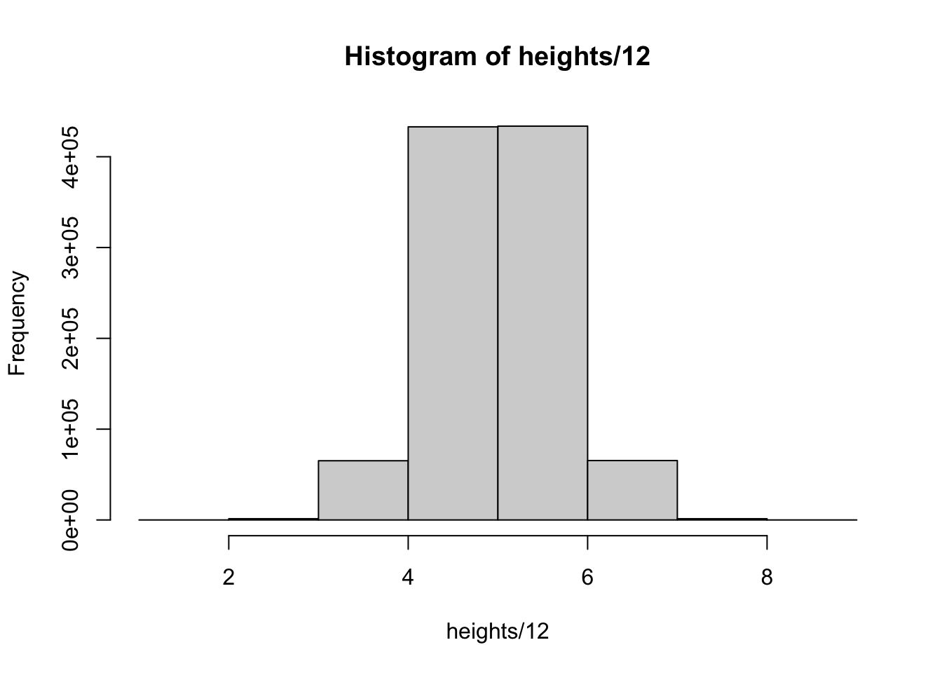
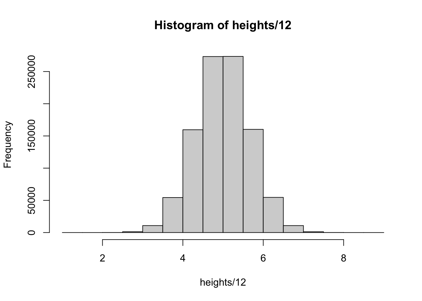
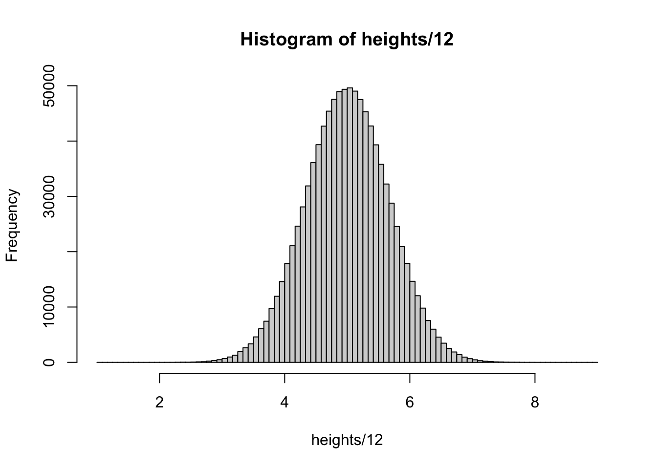
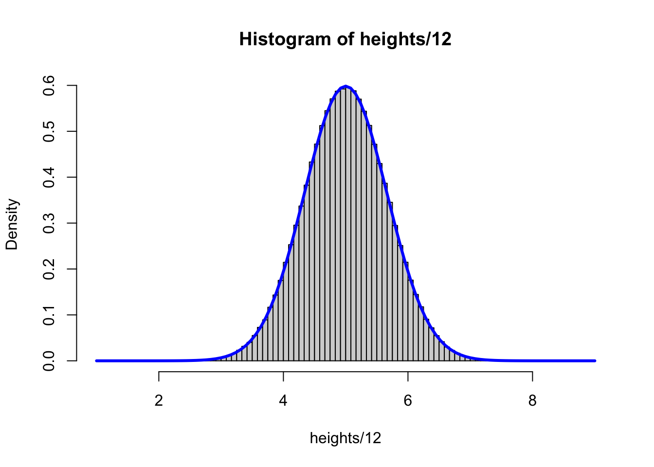
While we counted up the probability associated with different discrete parameters we can’t do that with continuous variables.
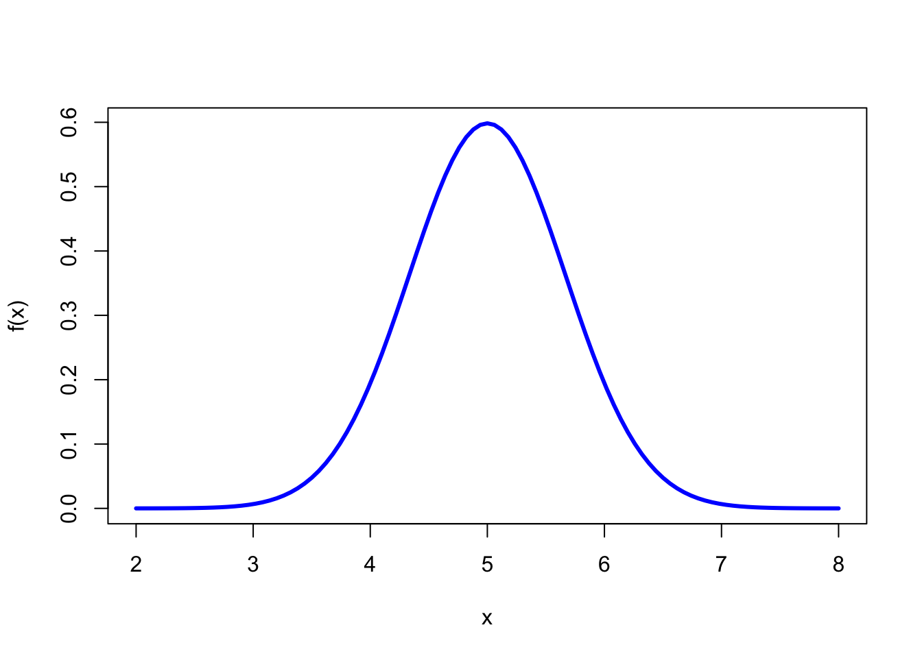
That curve is defined by a probability density function or pdf
In order to get probabilities, we need to look at areas under the curve:
For example, the probability that x is between 3 and 5 is equal to the area under this curve:
Just like the discrete probabilities, the area under the curve for the whole curve is 1.
The big difference is the probability of a specific number \(P(x = a) = 0\)
This implies the \(P(x \gt a) = P(x \ge a)\) and \(P(x \lt a) = P(x \le a)\)
Ex. If you are asking the probability of someone being 6 feet tall, what you really want to know is what’s the probability that they are greater than 5’11 1/2 and less than 6’0 1/2.
The next thing to deal with is what probability density function should you pick for your data? It’s not like with the discrete case where we could just list out the probabilities of specific number
Continuous Uniform Probability Distribution
\[ f(x) = \frac{1}{b - a} \text{ for } a \le x \le b \]
x can only run from a to b
a and *b are parameters
Notice that the distribution is constant - does not change no matter what value of x we plug in
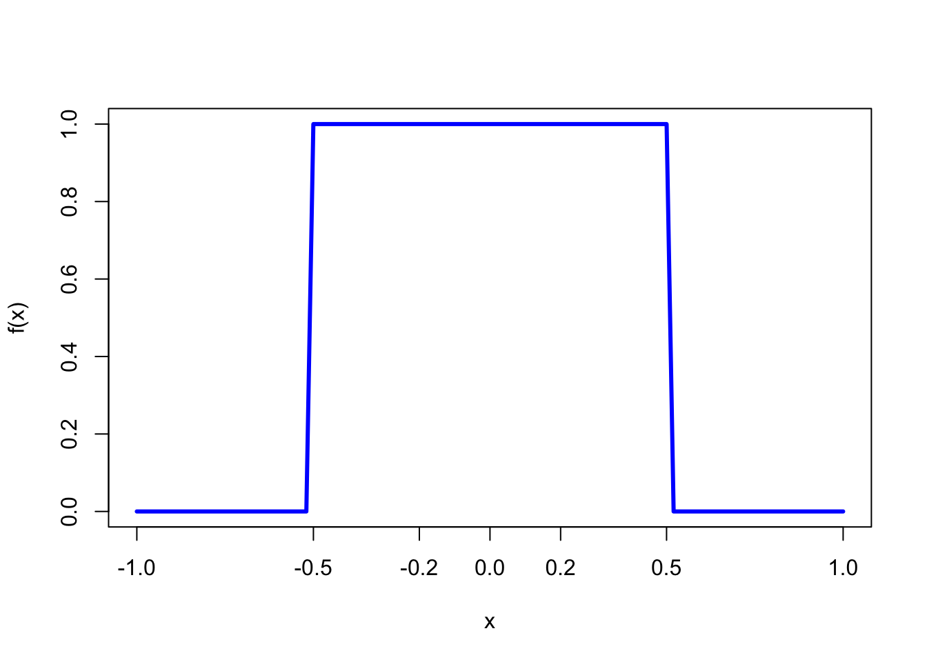
(Draw Figure 6.3) - Uniform Probability distribution
\[ \mu = \frac{b+a}{2} \]
Note: book has a typo that says \(b - a\). The formula above is correct for \(\mu\).
\[ \sigma^2 = \frac{(b - a)^2}{12} \]
Example 6.1
The error introduced by rounding an observation to the nearest inch has a uniform distribution over the interval from -.5 to .5. What is the probability that the rounding error is less than .2 in absolute value (i.e., \(-.2 \lt x \lt .2\))
The Exponential Probability Distribution
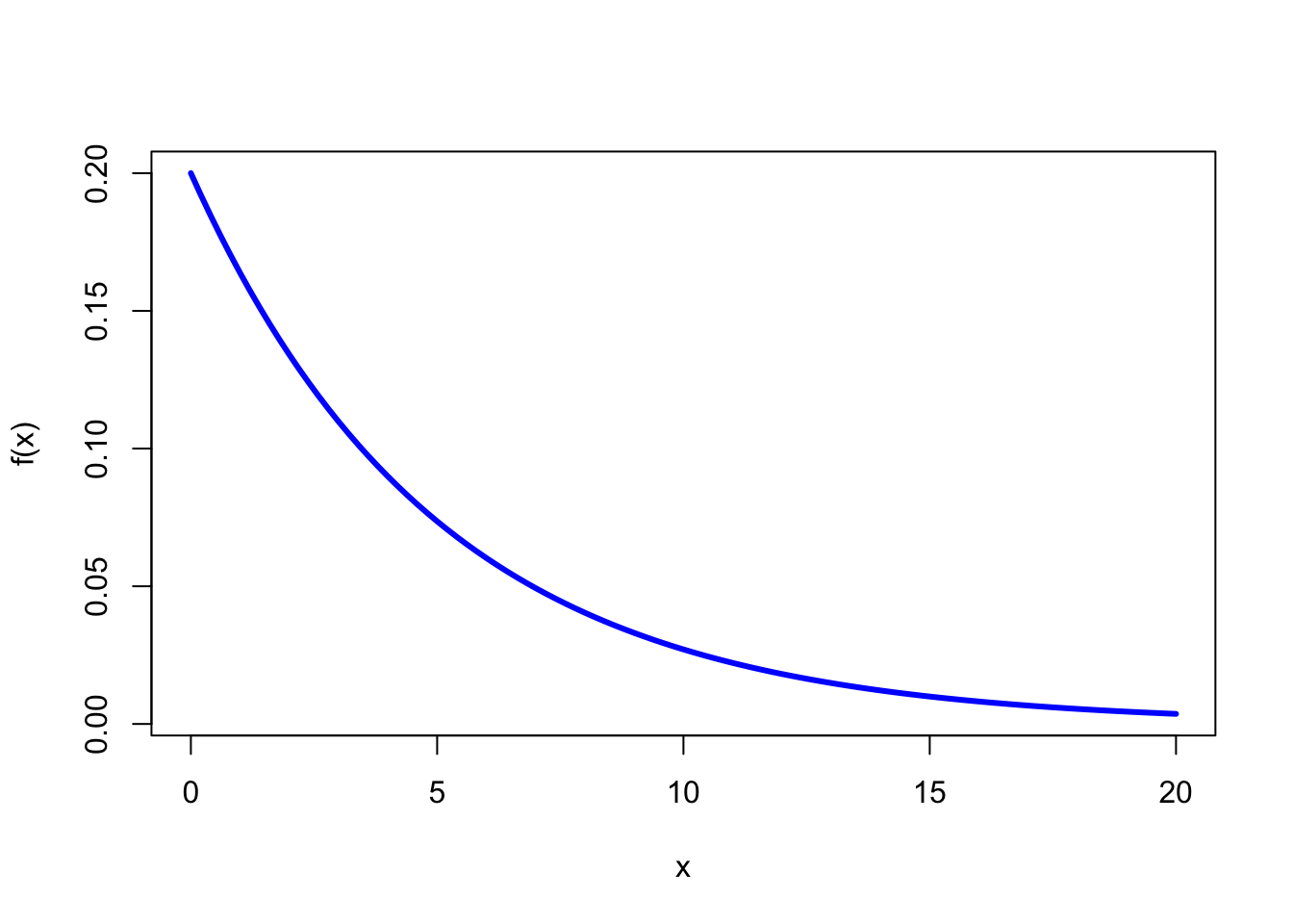
\[ f(x) = \lambda e^{-\lambda x} \text{ for } x \ge 0 \text{ and } \lambda > 0 \]
\(\mu = 1/\lambda\)
\(\sigma^2 = 1/\lambda^2\)
\[ P(x > a) = e^{-\lambda a} \]
Example 6.2
The waiting time at a supermarket checkout counter has an exponential distribution with an average waiting time of 5 minutes. What is the probability that you will have to wait more than 10 minutes at the checkout counter?
Here we are given \(\mu\) - what is \(\lambda\)?
Homework
[1] "6.1.18, 6.1.19"Answers: Section 6.1
Section 6.2 The Normal Probability Distribution
The normal probability distribution is a very common distribution because a lot of measurements follow this distribution at least approximately.
The pdf is defined by:
\[ f(x) = \frac{1}{\sigma \sqrt{2 \pi}} e^{-(x - \mu)^2/(2 \sigma^2)} \]
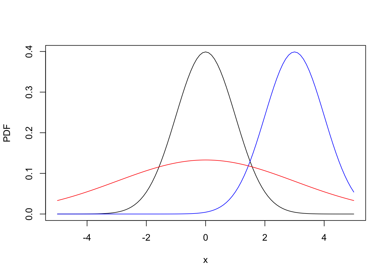
What are the parameters of the distribution?
Some example of normal distributions
The Standard Normal Random Variable
It can be challenging to calculate area under the curve for the normal distribution because of the infinite number of combinations of \(\mu\) and \(\sigma\).
We would need a separate table for each combination!
We can deal with this by standardizing the data we get to a z-score.
\[ z = \frac{x - \mu}{\sigma} \]
This is the equivalent of looking at a distribution that has \(\mu = 0\) and \(\sigma = 1\).
a portion of the table from the book is shown below.
Note that the rows show z to the 10ths place and the columns show the 100ths place of z.
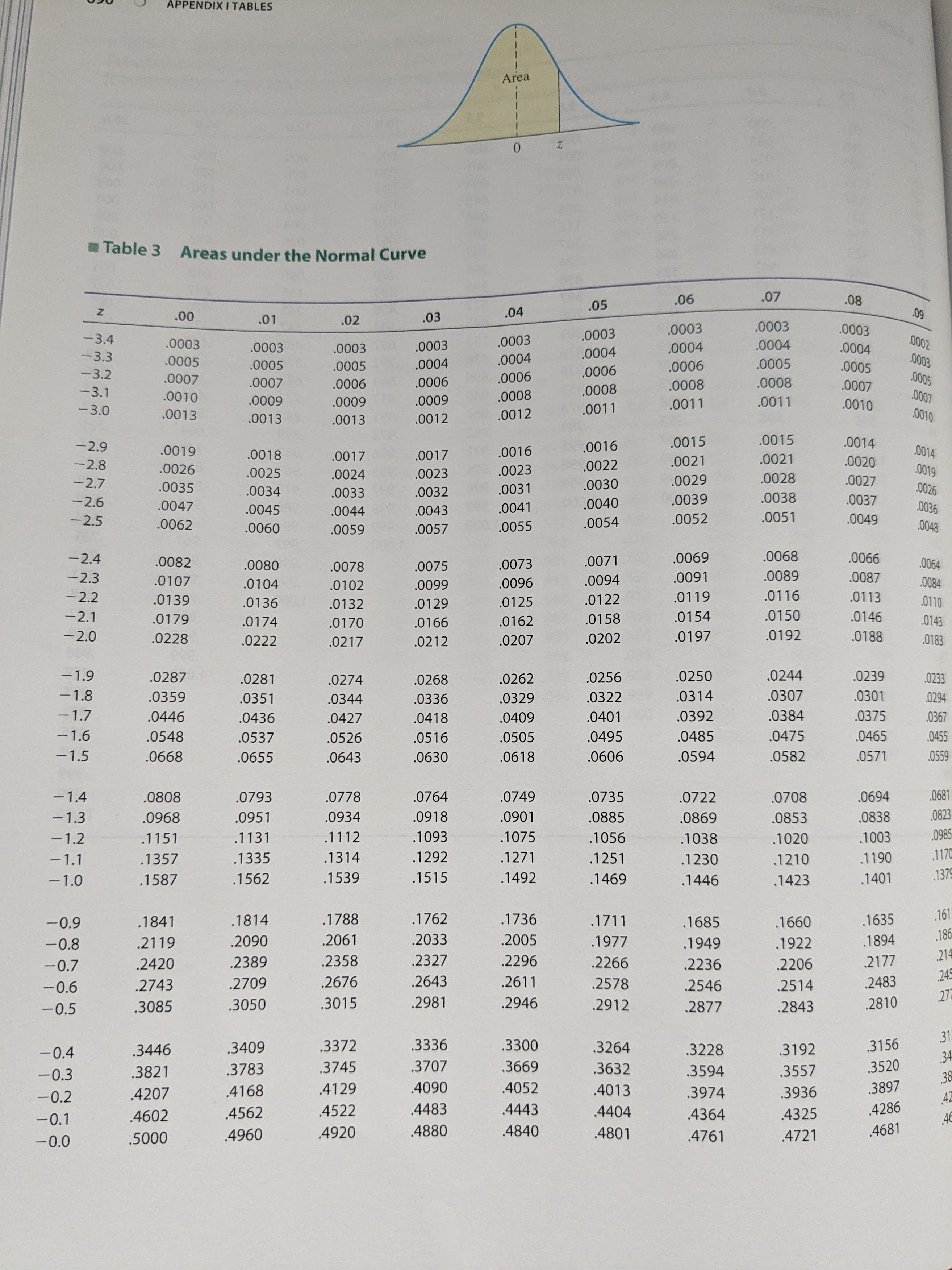
Find
\(P(z\le -1.96)\)
\(P(z\lt -1.96)\)
\(P(z\gt -1.96)\)
What about \(P(z > 1.96)\) ?
z-score can also be thought of as the number of standard deviations a number is from the mean.
Example 6.8
x is a normally distributed normal random variable with a mean of 10 and standard deviation of 2. Find the probability that x lies between 11 and 13.6?
\[ \begin{aligned} 11 \le& x \le 13.6 \\ 11 - 10 \le& x - 10 \le 13.6 - 10 \\ \frac{11 - 10}{2} \le& \frac{x - 10}{2} \le 13.6 - 10 \\ .5 \le& z \le 1.8 \end{aligned} \]
- show how this is the same using interactive tool
Example 6.9
Gas mileage for compact cars is normally distributed with mean of 35.5 mpg and std of 4.5.
What percentage of compacts get 40 mpg or more
Convert to z-score
Answer is 15.8%
Homework
[1] "6.2.46-48, 6.2.68"Answers: Section 6.2